Your Option Book Is a Knapsack Problem (The Hard Kind)

Deciding how much capital to commit to which option positions is a knapsack problem. Each candidate contract is an item with a value (the premium) and a weight (the loss it adds to the book under stress), and your risk budget is the capacity. The textbook version of that problem has a clean, provably optimal answer. The version an option book poses is multi-dimensional integer knapsack: whole contracts, as many as seven simultaneous capacities, and caps that apply to whole groups of items. That problem is NP-hard and has no efficient exact solution, so our premium optimizer answers it with a greedy heuristic that carries no guarantee it found the best plan.

The classic problem, briefly

You have a sack that holds ten kilograms and a pile of items, each with a weight and a value. Take the most valuable load that fits.

There are two versions, and the difference between them is the whole point.

In the fractional version you can take part of an item. Sort everything by value density (value divided by weight), take the densest first, then fill the last sliver with a fraction of whatever comes next. That greedy rule does not merely work well, it is provably optimal, with no search or backtracking anywhere in it.

In the 0/1 version you take each item whole or not at all. That one is NP-hard, but the friendly kind: a pseudo-polynomial dynamic program solves it, and a fully polynomial-time approximation scheme gets you inside any tolerance you name at predictable cost.

Hold on to the fractional result. Everything below is a way an option book departs from it.

Why a wheel book is exactly this problem

The mapping is tighter than an analogy. Value is the premium: each candidate contract, meaning one name at one strike for one expiry, collects a credit. Weight is the crash loss it adds, and the number that counts is the marginal one, how much more net liquidation value the book gives up in a reference bear market once this contract is on it. Not the contract's own max loss, which describes an event that never happens across a whole book at once. Capacity is the crash budget: you state the fraction of net liquidation value you will model losing in that drawdown, and the allocator may not exceed it.

That leaves the ranking, which is value density. The optimizer scores every candidate as premium bought per dollar of additional modelled crash loss, takes the highest, commits it, re-scores, and repeats. That is the greedy knapsack rule, though we arrived at it from the risk side rather than out of a textbook.

For any of this to be a knapsack, one thing has to hold: the weights have to add up. Net liquidation value is additive across legs, and the crash stress is a single-factor shock scaled per name, meaning one market drop with each name moving by a multiple derived from its own volatility, and volatility expanding as prices fall. There is no covariance matrix in there. So the running total of consumed capacity is a genuine sum, and it can be carried leg by leg without re-stressing the whole book each time.

Correlation still gets a say, just not there. It prices the score, penalising a candidate that duplicates exposure you already carry, and it decides which names reach the shortlist to begin with. It never touches the budget arithmetic, and that separation cost us a rewrite to learn. An earlier version let decorrelation into the risk denominator, and the allocator worked out almost immediately that it could win on value density by shrinking the denominator instead of earning premium. What came back was a plan full of quiet, low-volatility names that collected very little and scored beautifully.

The mechanics of the search are covered separately; this piece is about why the problem is hard.

Break one: you sell whole contracts

The fractional knapsack is the one case where greedy is exactly optimal, and it is the one case options can never be. An option contract is 100 shares of deliverable. There is no half a put.

So the allocator adds one contract at a time and counts in whole numbers, which drops the problem into the 0/1 family: NP-hard, and no longer a case where sorting by density is the answer.

"Integers" undersells how lumpy this gets. One contract on a $400 strike commits $40,000 of collateral. Against a per-name notional cap set as a percentage of net asset value, the difference between two contracts and three is often the difference between fitting and not fitting, with nothing available in between. A solver free to take 2.4 contracts would happily find allocations that do not exist in the tradeable set.

Break two: seven capacities, not one

This is where the friendly kind of NP-hard ends. A candidate is not checked against one budget but against as many as seven, and it has to clear every one of them that is live:

• the per-name contract cap
• the per-name notional cap, as a percentage of net asset value
• the deployable-cash pool, when the run is bounded by one
• the release-concentration cap, limiting how much collateral may free in any single week, off by default
• the crash budget
• the volatility-shock budget, off by default
• the expected-assignment budget, in dollars of stock you should expect to be handed

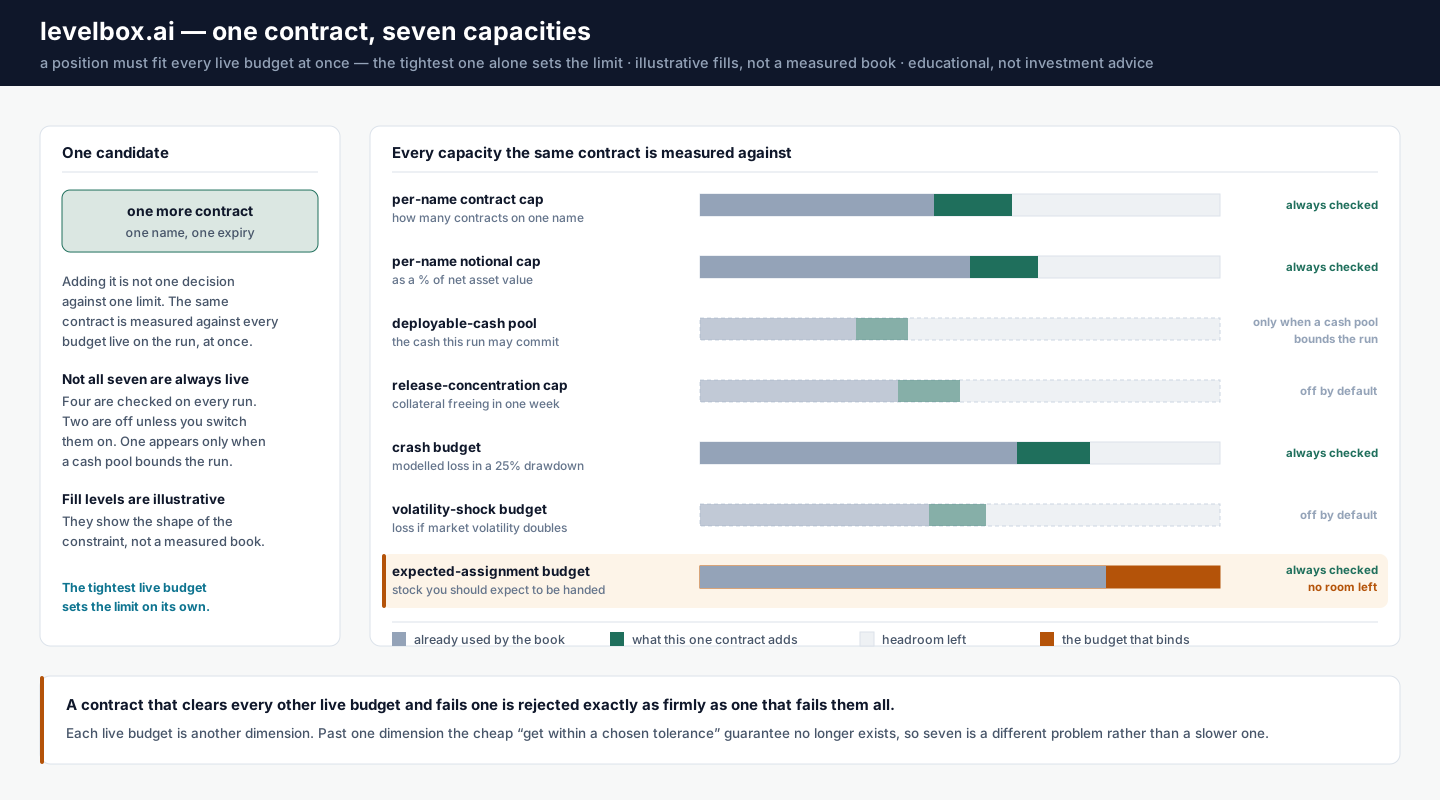
That is multi-dimensional knapsack, and the difficulty does not scale gently. The one-dimensional case has a fully polynomial approximation scheme: name a tolerance, reach it at predictable cost. From two dimensions up, no fully polynomial scheme exists unless P equals NP, and the usual "just get within one percent cheaply" escape hatch goes with it. So seven dimensions is not seven times harder than one. It is a different problem with the convenient result deleted.

Stacking gates is expensive too, which is why they run in cost order: cheap arithmetic first, the ones that need a marginal re-valuation of the book last.

Break three: the items come in classes

The per-name caps add a third departure. A cap on this contract is an ordinary weight. A cap on every contract sharing an underlying is a constraint on a group of items, which means feasibility becomes a property of the whole set you have chosen so far rather than a running sum you can check one item against.

The group caps are not constants either. The cap governs concurrent exposure, so what an existing short put consumes against a new candidate depends on how much of the candidate's life the two actually overlap. A put expiring tomorrow should not reserve the same slice of a name's capacity against a 30-day candidate as one with 30 days left on it. The caps are therefore seeded per candidate expiry and weighted by that overlap, weighted rather than switched by a yes/no test, because a boolean puts a cliff right at the boundary: a 29-day leg would drop to zero consumption against a 30-day candidate it coexists with for 29 of those 30 days.

Which means a name's remaining room differs by expiry, and there is no single number you can point at for what is left.

What greedy gives up

Greedy commits and never revisits, and that is the whole of what it costs.

The failure mode is easy to picture. Several small, high-density picks taken early eat a budget that one larger position would have used better, and the allocator has no way to unwind three cheap contracts to make room for a better one it meets later. In the textbook 0/1 problem, density-greedy's worst case is unboundedly bad: one tiny item with excellent density can crowd out the single item that would have filled the sack.

A real allocation is not that worst case. Hundreds of candidates across many names and expiries, added one contract at a time, is a far better-behaved surface than something an adversary built to break you. But "not the worst case" is not a bound, and the gap between what the allocator returns and the true optimum is unmeasured. Measuring it would mean solving the exact problem the heuristic exists to avoid, on every run, in a setting where scoring one candidate means re-valuing a whole book under stress.

One thing worth separating out, because the two get conflated. The allocator is fast because per-leg valuations are memoised and running totals are carried incrementally rather than re-summed. Both of those are exact, so none of that speed costs accuracy. The approximation lives entirely in the search order, in which candidate gets taken next and in the fact that the choice is never reconsidered.

"No answer" is a real answer

Several simultaneous budgets can leave an empty feasible set. Nothing fits, and the correct output is a plan with no trades in it.

Most tools would rather show you something. An empty plan reads as a broken optimizer unless the tool tells you why it is empty, so most of the work here went into naming which budget stopped it, and then into naming every cause that rejected a candidate on the final pass, largest first, each with its own count.

Reporting only the largest cause was the original behaviour, and it could tell you something false. Suppose a volatility budget truncates a plan, and it and a per-name notional cap each reject exactly one candidate. A largest-cause report breaks that tie arbitrarily and announces that the notional cap truncated the plan, which it did not. For an analytical product a false cause is worse than a vague one, so it had to go.

The verdict also distinguishes "no candidate cleared" from "the plan was truncated", and it comes back as machine-readable keys alongside the sentence, so an interface can mark the exact control that bound rather than leaving you to hunt for it in a paragraph.

An empty plan under budgets you set yourself is information: your constraints are mutually infeasible, and you now know which pair to argue with.

Where this is rough today

The optimizer is a work in progress, and this is the claim I would defend for it: useful for comparing choices, not precise enough to treat as a measurement. This budget against that one, this delta against that one, premium and risk on the same clock: those comparisons hold up. The absolute level does not. A model that ranks alternatives correctly while getting the level wrong is still worth having. It just is not a number you can go and quote at someone.

Modesty in the abstract is worth less than the list behind it, so here is the list, as of publication.

No optimality guarantee, and the gap is unmeasured. Covered above. It is the biggest caveat here.

Three of our own code paths once disagreed about the same book's crash loss by roughly ten percentage points. Each had independently pinned market volatility to a hardcoded constant instead of reading it off the market. That is fixed, and they now land within about two points of each other, but we still do not claim any one of the three is right. Read the spread as a floor on how wrong the model can be rather than as a confidence interval.

Positions held only as short puts get a fabricated underlying price. The statement we read does not carry a spot, so the price is derived from the strike on a fixed out-of-the-money assumption. Checked against live quotes it came in 15–39% low on the names we looked at, which puts those positions closer to the money than they really are and so overstates the tail. About half the positions in the book we test against are affected. Still open.

A hand-maintained volatility table understated every name we could measure it against, several by more than double, and understating a name's volatility understates how far it moves in the modelled crash. Live readings come first now, so the table is a fallback. It has not gone away, though. A name with no fresh reading still lands on it, and a proxy-sourced volatility is closer to a floor than an estimate.

The crash figures are our own conservative model, not a broker's. They will not match your margin engine, and they are not meant to.

---

The reason the knapsack framing is worth the detour is that it tells you which properties to want. Exactness is not one of them at this problem size. It is not available, and anyone claiming it is either solving a smaller problem or has not checked. What you can have is a stated objective, budgets you set yourself, an explicit price on every pick, and a tool that tells you when your constraints cannot all hold instead of quietly choosing one to ignore.

Analytical and educational tooling, not investment advice. Crash figures come from our own conservative margin model rather than your broker's, and assignment probabilities are risk-neutral quantities rather than forecasts. Assignment is the intended mechanism of a cash-secured put, not a failure of one; the risk being modelled is a name that keeps falling. Options carry the risk of loss — work through the numbers on your own book and decide for yourself.